Prophet: A Hidden Seasonality Bug


Prophet is widely recognized for its automatic parameter fitting, which makes time series forecasting accessible without extensive manual tuning. This is especially attractive when working with many time series at once, where carefully supervising each individual model is simply not feasible.
Relying on this automation and its popularity, we chose Prophet as our main forecasting tool for a large-scale prediction task. Yet we quickly ran into a puzzling issue: some models trained on similar data behaved very differently, with certain runs producing sensible forecasts and others failing dramatically. These inconsistent outcomes raised a key question: what exactly was driving such unstable behavior?
A puzzling case: Prophet Misfits.
To investigate this, imagine you are forecasting hundreds or thousands of series with Prophet and cannot inspect them one by one. When you randomly sample a few forecasts, some of them look completely wrong. To make this situation concrete, throughout this post we will work with a well-known dataset bundled with Prophet: the daily log page views of Peyton Manning’s Wikipedia page.
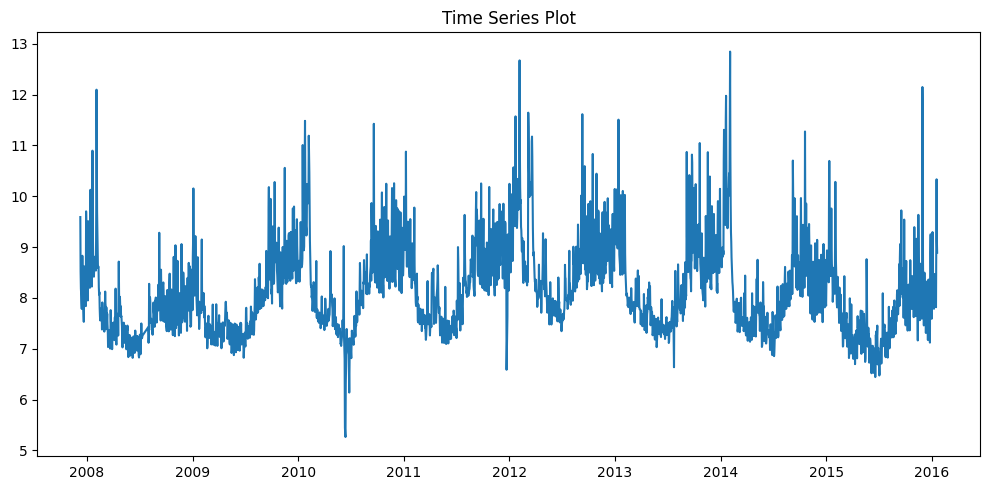
This series is deliberately chosen because it is highly structured and visually “forecastable”; in fact, it appears in Prophet’s own documentation as a canonical example of multiple seasonalities and trend changes. Using this dataset, we will reproduce and analyze the bug, starting by defining a helper function to fit the model and visualize its forecasts in a consistent manner.
# Auxiliary to plot and fit
def train_and_plot_model(train, test, model):
    model.fit(train)  # train

    future = model.make_future_dataframe(periods=len(test), freq='D')
    forecast = model.predict(future)  # predict

    test_forecast = forecast.iloc[-len(test):]
    mae = np.mean(np.abs(test['y'].values - test_forecast['yhat'].values))

    fig = plot_plotly(model, forecast)

    return test_forecast, mae, fig
This helper takes a training set, a test set, and a Prophet model, fits the model, produces a forecast over the whole horizon, computes a simple MAE on the test window, and returns both the forecast and a Plotly figure. Now that we have a small utility to train, forecast, and visualize, we can plug in the Peyton Manning dataset.
# Example data read
link_dataset = 'https://raw.githubusercontent.com/facebook/prophet/main/examples/example_wp_log_peyton_manning.csv'
polars_df = pl.read_csv(link_dataset).with_columns(pl.col('ds').str.to_date())

# split into train and test
df = polars_df.to_pandas()
train_polars = df.iloc[:-300].copy()
test_polars = df.iloc[-300:].copy()

# fit model
model_polars = Prophet()
forecast_polars, mae_polars, fig_polars = train_and_plot_model(train_polars,
                     test_polars,
                     model_polars
)
fig_polars.show()
This code loads the dataset, splits it into training and test sets, trains a default Prophet model on the training data and generates forecasts.
From the code alone, everything follows the usual Prophet pattern: i) fit on the historical data, ii) extend the horizon with make_future_dataframe, and iii) evaluate using a simple MAE. Yet, as the plot below shows, the resulting forecast is completely off, even on the training period! This is our first clue that something deeper is wrong.
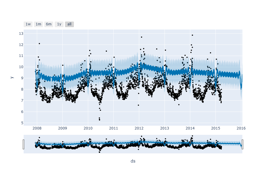
Concerned, you conduct an exhaustive test across your entire dataset, only to discover that the evaluation metrics suggest the models are performing well. What’s going on?
Lets go back to the simplest approach: replicate exactly what the Prophet Quick start guide uses.
This is the standard, documented way to use Prophet, and if the bug exists even here, it reveals a fundamental flaw in the library itself.
# Read
pandas_df = pd.read_csv(link_dataset)
# by default this dataset read the time column as Object.
pandas_df['ds'] = pd.to_datetime(pandas_df['ds'])

# Split
train_pandas = pandas_df.iloc[:-300].copy()
test_pandas = pandas_df.iloc[-300:].copy()

# Train
model_pandas = Prophet()
forecast_pandas, mae_pandas, fig_pandas = train_and_plot_model(train_pandas,
                                                           test_pandas,
                                                           model_pandas
                                                           )
The results are dramatically different: both past values and future forecasts are now accurate. Here is an overlapped predictions plot below, where you can see the stark contrast—where the Polars-processed model failed catastrophically, the pandas-processed model succeeds perfectly.
The only difference between the two approaches is how the data is loaded—yet this single change produces dramatically different predictions. How is this even possible? The Polars-processed data and pandas-processed data generate completely opposite results, despite the data values appearing identical when compared:
assert (train_pandas == train_polars).all().all()
assert (test_pandas == test_polars).all().all()To understand what went wrong, we need to examine Prophet’s internal implementation. The bug must be in how Prophet processes the data, not in the data itself.
Prophet’s Components: A Quick Refresher
Prophet decomposes time series forecasts into four key components:
- Trend: The long-term direction of the data
- Seasonality: Recurring patterns that repeat at fixed intervals (daily, weekly, yearly)
- Regressors: Additional external variables that influence the forecast
- Confidence Interval: Uncertainty bounds around predictions
Regressors are not being used, but we can examine the other three components in the following plot:
The trend and confidence intervals look reasonable: similar for both examples, with only a small shift. However, the seasonality component tells a completely different story—it looks dramatically different between the two approaches. This may be the key to understanding what went wrong.
Finding the Seasonality
We have to dig deeper into Prophet’s internals to understand where the seasonality detection was failing. The bug had to be somewhere in how Prophet computes its seasonality features.
Let’s examine Prophet’s seasonality functions, found in the file prophet/python/prophet/forecaster.py:
@classmethod
def make_seasonality_features(cls, dates, period, series_order, prefix):
    """Data frame with seasonality features.

    Parameters
    ----------
    cls: Prophet class.
    dates: pd.Series containing timestamps.
    period: Number of days of the period.
    series_order: Number of components.
    prefix: Column name prefix.

    Returns
    -------
    pd.DataFrame with seasonality features.
    """
    features = cls.fourier_series(dates, period, series_order)
    columns = [
        '{}_delim_{}'.format(prefix, i + 1)
        for i in range(features.shape[1])
    ]
    return pd.DataFrame(features, columns=columns)
Everything looks fine in here, lets take a look on how the fourier series are computed in the method fourier_series:
# Prophet's seasonality detection code
@staticmethod
def fourier_series(
    dates: pd.Series,
    period: Union[int, float],
    series_order: int,
) -> NDArray[np.float64]:
    """Provides Fourier series components with the specified frequency
    and order.

    Parameters
    ----------
    dates: pd.Series containing timestamps.
    period: Number of days of the period.
    series_order: Number of components.

    Returns
    -------
    Matrix with seasonality features.
    """
    if not (series_order >= 1):
        raise ValueError("series_order must be >= 1")

    # convert to days since epoch
    t = dates.to_numpy(dtype=np.int64) // NANOSECONDS_TO_SECONDS / (3600 * 24.)

    x_T = t * np.pi * 2
    fourier_components = np.empty((dates.shape[0], 2 * series_order))
    for i in range(series_order):
        c = x_T * (i + 1) / period
        fourier_components[:, 2 * i] = np.sin(c)
        fourier_components[:, (2 * i) + 1] = np.cos(c)
    return fourier_components
This function transforms timestamps into sine and cosine features that capture seasonal patterns. Here’s how it works:
-
Convert timestamps (since epoch) to integer values:
t = dates.to_numpy(dtype=np.int64) // NANOSECONDS_TO_SECONDS / (3600 * 24.) -
Scale time to radians:
x_T = t * np.pi * 2 -
Generate sine and cosine pairs:
 for i in range(series_order):
     c = x_T * (i + 1) / period
     fourier_components[:, 2 * i] = np.sin(c)
     fourier_components[:, (2 * i) + 1] = np.cos(c)
At first glance, this looks solid. But then we noticed something: What is NANOSECONDS_TO_SECONDS constant doing there?
The Root Cause
We found it. In Prophet’s initialization code, there’s a constant that reveals the root cause:
# Show the hardcoded time unit dependency
...
logger = logging.getLogger('prophet')
logger.setLevel(logging.INFO)
NANOSECONDS_TO_SECONDS = 1000 * 1000 * 1000

class Prophet(object):
    stan_backend: IStanBackend

    """Prophet forecaster.
....
NANOSECONDS_TO_SECONDS is defined as 1000 * 1000 * 1000 (10⁹), a conversion factor from nanoseconds to seconds.
When you call dates.to_numpy(dtype=np.int64), pandas converts the date Series into an array of integers representing time since the Unix epoch. The actual magnitude of these integers depends on the datetime resolution of your data. If your timestamps are stored as datetime64[ns] (nanoseconds), integers represent nanoseconds, but if they are datetime64[us], they represent microseconds.
Prophet doesn’t consider this. It blindly divides by NANOSECONDS_TO_SECONDS regardless of your timestamp resolution. When the data is in microseconds (or in a different unit: milliseconds, seconds…), dividing by 10⁹ produces values 1000 times smaller (or even to lower scales). This scaled float series implies that the Fourier features become corrupted, and seasonality detection silently fails with no errors, no warnings, just wrong results.
This nanosecond dependency is not documented anywhere in Prophet’s official documentation or API reference. Users are expected to know this implementation detail, yet there’s no warning or mention of it in the guides or docstrings. This represents a critical vulnerability in Prophet’s design: when the assumption about datetime precision is violated, the model completes training without raising any errors or warnings, while silently producing inaccurate predictions.
The Bug Revealed
When we checked our data sources, did they have different data resolution? Yes
print(f"Pandas dtype: {pandas_df['ds'].dtype}")
print(f"Polars dtype: {df['ds'].dtype}")Pandas dtype: datetime64[ns] Polars dtype: datetime64[us]
Polars’ default microsecond precision is preserved when converting to pandas with .to_pandas(), while pandas’ native pd.to_datetime() uses nanoseconds. This difference invisible to fast equality checks breaks Prophet’s seasonality detection (as Prophet assumes nanoseconds, causing 1000x compression in Fourier features).
assert pandas_df['ds'].dtype == df['ds'].dtype, 'wrong dtype'Pandas: datetime64[ns]
Polars: datetime64[us]
Reminder: Python’s equality operator for dataframes does not check dtypes. To properly validate use .equals() to catch dtype mismatches that can break Prophet.
pandas_df.equals(df)Result: False
Quick solutions: Either ensure that you match the resolution of nanoseconds so that Prophet will correctly compute Fourier features for seasonality detection…
# Fix: Ensure datetime64[ns] resolution
df['ds'] = df['ds'].astype('datetime64[ns]')Fixed dtype: datetime64[ns]
… Or upgrade to the latest version of Prophet.
Pandas 3.0 and Prophet 1.3.0
By the time this post was published, Pandas 3.0 was released. Pandas 3.0 removed the default datetime64[ns] resolution.
Prophet 1.3.0 adapted to this by updating the epoch conversion logic, following pandas documentation recommendations:
# New approach in Prophet 1.3.0
epoch = pd.Timestamp("1970-01-01", tz=dates.dt.tz)
t = (dates - epoch).dt.total_seconds() / (24 * 60 * 60)
This new approach automatically handles any datetime resolution without making assumptions, a fix that should have been in place from the beginning. However, Prophet’s response reveals a critical flaw in its design philosophy: the library was built with implicit assumptions about its input data that were never validated or documented. The NANOSECONDS_TO_SECONDS constant remains defined in the codebase, though it’s no longer used. Some related GitHub issues remain open, suggesting this fix may not be widely known yet.
Replicability Environment Details
- Prophet version: [<=1.2.2]
- Pandas version: [<3.0]